Record linker
The record linker tool matches structured query records to a fixed set of reference records with the same schema. A common example of this is matching address records from a query dataset to a relatively error-free reference address database.
To illustrate this example with the record linker tool, we use synthetic address data generated by and packaged with the FEBRL program, another data matching tool. For the sake of illustration suppose the set called "refs" is a clean set of reference addresses (say, from a government collected and curated database), while the SFrame called "query" contains new data with many errors.
import os
import graphlab as gl

col_types = {'street_number': str, 'postcode': str}

if os.path.exists('febrl_F_org_5000.csv'):
    refs = gl.SFrame.read_csv('febrl_F_org_5000.csv',
                              column_type_hints=col_types)
else:
    url = 'http://s3.amazonaws.com/dato-datasets/febrl_synthetic/febrl_F_org_5000.csv'
    refs = gl.SFrame.read_csv(url, column_type_hints=col_types)
    refs.save('febrl_F_org_5000.csv')

if os.path.exists('febrl_F_dup_5000.csv'):
    query = gl.SFrame.read_csv('febrl_F_dup_5000.csv',
                               column_type_hints=col_types)
else:
    url = 'http://s3.amazonaws.com/dato-datasets/febrl_synthetic/febrl_F_dup_5000.csv'
    query = gl.SFrame.read_csv(url, column_type_hints=col_types)
    query.save('febrl_F_dup_5000.csv')
For simplicity, we'll discard several of the features right off the bat. The
remaining features have the same schema in both the refs and query SFrames.
Note the large number of errors present even in the first few rows of the query
dataset.
address_features = ['street_number', 'address_1', 'suburb', 'state', 'postcode']
refs = refs[address_features]
query = query[address_features]

refs.head(5)
+---------------+---------------------+---------------+-------+----------+
| street_number |      address_1      |     suburb    | state | postcode |
+---------------+---------------------+---------------+-------+----------+
|       95      |     galway place    |    st marys   |       |   2681   |
|       12      |    burnie street    |   wycheproof  |  nsw  |   2234   |
|       16      | macrobertson street |    branxton   |  qld  |   3073   |
|      170      |    bonrook street   | brighton east |  nsw  |   3087   |
|       32      |   proserpine court  |   helensvale  |  qld  |   2067   |
+---------------+---------------------+---------------+-------+----------+
[5 rows x 5 columns]
query.head(5)
+---------------+-----------------+-------------------+-------+----------+
| street_number |    address_1    |       suburb      | state | postcode |
+---------------+-----------------+-------------------+-------+----------+
|       31      |                 |     reseevoir     |  qld  |   5265   |
|      329      |                 | smithfield plains |  vic  |   5044   |
|       37      | kelleway avenue |     burwooast     |  nsw  |   2770   |
|       15      |  mawalan street |     kallangur     |  nss  |   2506   |
|      380      |   davisktrdet   |    boyne ilsand   |  nss  |   6059   |
+---------------+-----------------+-------------------+-------+----------+
[5 rows x 5 columns]
Basic usage
The record linker model is somewhat smart about what feature transformations are needed to accommodate the specified distance (although note that the street number and postcode fields had to be forced to strings when the datasets were imported). For our first pass, we'll use Jaccard distance, which implicitly concatenates all features (as strings), then converts them to character n-grams (a.k.a. shingles). In our experience, this is a good strategy for obtaining reasonable first results from address features.
model = gl.record_linker.create(refs, features=address_features,
                                distance='jaccard')
model.summary()
Class                               : RecordLinker

Schema
------
Number of examples                  : 3000
Number of feature columns           : 5
Number of distance components       : 1
Method                              : brute_force

Training
--------
Total training time (seconds)       : 2.7403
Results are obtained with the model's link method, which matches a new set
of queries to the reference data passed in above to the create function. For
our first pass, we set the radius parameter to 0.5, which means that matches
must share at least roughly 50% of the information contained in both the
reference and query records.
matches = model.link(query, k=None, radius=0.5)
matches.head(5)
+-------------+-----------------+-----------------+------+
| query_label | reference_label |     distance    | rank |
+-------------+-----------------+-----------------+------+
|      1      |       2438      |  0.41935483871  |  1   |
|      1      |       533       |       0.5       |  2   |
|      2      |       688       |  0.192307692308 |  1   |
|      3      |       2947      | 0.0454545454545 |  1   |
|      5      |       1705      |  0.047619047619 |  1   |
+-------------+-----------------+-----------------+------+
[5 rows x 4 columns]
The results mean that the address in query row 1 match the address in refs
row number 2438, although the Jaccard distance is relatively high at 0.42.
Inspecting these records manually we see this is in fact not a good match.
print query[1], '\n'
print refs[2438]
{'suburb': 'smithfield plains', 'state': 'vic', 'address_1': '',
'street_number': '329', 'postcode': '5044'}

{'suburb': 'smithfield plains', 'state': 'vic', 'address_1': 'sculptor street',
'street_number': '16', 'postcode': '5044'}
On the other hand, the match between query number 3 and reference number 2947 has a distance of 0.045, indicating these two records are far more similar. By pulling these records we confirm this to be the case.
print query[3], '\n'
print refs[2947]
{'suburb': 'kallangur', 'state': 'nss', 'address_1': 'mawalan street',
'street_number': '15', 'postcode': '2506'}

{'suburb': 'kallangur', 'state': 'nsw', 'address_1': 'mawalan street',
'street_number': '12', 'postcode': '2506'}
Defining a composite distance
Unfortunately, these records are still not a true match because the street numbers are different (in a way that is not likely to be a typo). Ideally we would like street number differences to be weighted heavily in our distance function, while still allowing for typos and misspellings in the street and city names. To do this we can build a composite distance function.
A composite distance is simply a weighted sum of standard distance functions, specified as a list. Each element of the list contains three things:
- a list or tuple of feature names,
- a standard distance name, and
- a multiplier for the standard distance.
Please see the documentation for the GraphLab Create distances module for more on composite distances.
In this case we'll use Levenshtein distance to measure the dissimilarity in street number, in addition to our existing Jaccard distance measured over all of the address features. Both of these components will be given equal weight. In the summary of the created model, we see the number of distance components is now two---Levenshtein and Jaccard distances---instead of one in our first model.
address_dist = [
                [['street_number'], 'levenshtein', 1],
                [address_features, 'jaccard', 1]
               ]

model = gl.record_linker.create(refs, distance=address_dist)
model.summary()
Class                               : RecordLinker

Schema
------
Number of examples                  : 3000
Number of feature columns           : 5
Number of distance components       : 2
Method                              : brute_force

Training
--------
Total training time (seconds)       : 0.4789
One tricky aspect of using a composite distance is figuring out the best
threshold for match quality. A simple way to do this is to first return a
relatively high number of matches for each query, then look at the distribution
of distances for good thresholds using the radius parameter.
pre_match = model.link(query, k=10)
pre_match['distance'].show()
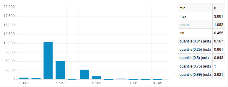
In this distribution we see a stark jump at 0.636 in the distribution of
distances for the 10-nearest neighbors of every query (remember this is no
longer simple Jaccard distance, but a sum of Jaccard and Levenshtein distances
over different sets of features). In our final pass, we set the k parameter to
None, but enforce this distance threshold with the radius parameter.
matches = model.link(query, k=None, radius=0.64)
matches.head(5)
+-------------+-----------------+----------------+------+
| query_label | reference_label |    distance    | rank |
+-------------+-----------------+----------------+------+
|      6      |       1266      | 0.333333333333 |  1   |
|      7      |       2377      | 0.208333333333 |  1   |
|      9      |       2804      | 0.575757575758 |  1   |
|      12     |       2208      | 0.181818181818 |  1   |
|      13     |       1346      | 0.111111111111 |  1   |
+-------------+-----------------+----------------+------+
[5 rows x 4 columns]
There are far fewer results now, but they are much more likely to be true matches than with our first model, even while allowing for typos in many of the address fields.
print query[6], '\n'
print refs[1266]
{'suburb': 'clayton south', 'state': '', 'address_1': 'ingham oace',
'street_number': '128', 'postcode': '7520'}

{'suburb': 'clayton south', 'state': 'nsw', 'address_1': 'ingham place',
'street_number': '128', 'postcode': '7052'}
References
- Febrl - A Freely Available Record Linkage System with a Graphical User Interface. Peter Christen. Proceedings of the ‘Australasian Workshop on Health Data and Knowledge Management’ (HDKM). Conferences in Research and Practice in Information Technology (CRPIT), vol. 80. Wollongong, Australia, January 2008.