Examples
To illustrate some of these methods, we'll use a previously created SGraph where vertices represent Wikipedia articles about US businesses and edges represent hyperlinks between articles. This data is available under the Creative Commons Attribution-ShareAlike 3.0 Unported License (more details here: http://en.wikipedia.org/wiki/Wikipedia:Copyrights). It can be downloaded from Dato's public datasets bucket on Amazon S3. The remaining methods are left for the reader to explore in the exercises at the end of the chapter.
import os

data_file = 'US_business_links'
if os.path.exists(data_file):
    sg = graphlab.load_sgraph(data_file)
else:
    url = 'http://s3.amazonaws.com/dato-datasets/' + data_file
    sg = graphlab.load_sgraph(url)
    sg.save(data_file)

print sg.summary()
{'num_edges': 517127, 'num_vertices': 233121}
PageRank
PageRank is an iterative algorithm to compute the most influential nodes in a network. In each iteration, a vertex's influence is measured as the sum of influence of the nodes that point at the vertex. Each node's score is updated until the scores converge, or until the user-specified maximum number of iterations is reached.

"PageRank-hi-res". Licensed under Creative Commons Attribution-Share Alike 2.5 via Wikimedia Commons - http://commons.wikimedia.org/wiki/File:PageRank-hi-res.png#mediaviewer/File:PageRank-hi-res.png
As with other GraphLab Create methods, the model object is constructed with the
create function. The summary() method provides a snapshot of the result, and
the list_fields() indicates the attributes of the model that can be queried.
pr = graphlab.pagerank.create(sg, max_iterations=10)
print pr.summary()
PagerankModel
Graph:
+--------------+--------+
| num_edges    | 517127 |
| num_vertices | 233121 |
+--------------+--------+
Result:
+----------+-------------------------------------------------------+
| graph    | SGraph. See m['graph']                                |
| pagerank | SFrame with each vertex's pagerank. See m['pagerank'] |
| delta    | 3824.08346598                                         |
+----------+-------------------------------------------------------+
Setting:
+-------------------+------+
| threshold         | 0.01 |
| reset_probability | 0.15 |
| max_iterations    | 10   |
+-------------------+------+
Metric:
+----------------+----------+
| num_iterations | 10       |
| training_time  | 7.223114 |
+----------------+----------+
Queriable Fields
+-------------------+-----------------------------------------------------------+
| Field             | Description                                               |
+-------------------+-----------------------------------------------------------+
| training_time     | Total training time of the model                          |
| graph             | A new SGraph with the pagerank as a vertex property       |
| delta             | Change in pagerank for the last iteration in L1 norm      |
| reset_probability | The probablity of randomly jumps to any node in the graph |
| pagerank          | An SFrame with each vertex's pagerank                     |
| num_iterations    | Number of iterations                                      |
| threshold         | The convergence threshold in L1 norm                      |
| max_iterations    | The maximun number of iterations to run                   |
+-------------------+-----------------------------------------------------------+
The model fields are retrieved either with the get method or by treating the
model as a dictionary, as in the following snippet which shows the model
creation run time of about 7 seconds.
print pr['training_time']
7.234136
The pagerank field contains an SFrame with the per-node pagerank score. For
this example of Wikipedia articles and hyperlinks, ABC takes the top spot by a
large margin.
pr_out = pr['pagerank']
print pr_out.topk('pagerank', k=10)
+-------------------------------+---------------+---------------+
|              __id             |    pagerank   |     delta     |
+-------------------------------+---------------+---------------+
| American Broadcasting Company | 3050.12285481 | 171.095519607 |
|           Microsoft           | 1640.93294801 | 79.4193105615 |
|           DC Comics           | 1623.76580168 |  231.05676926 |
|       Paramount Pictures      | 1341.29716993 | 74.7486642804 |
|            Facebook           | 1218.69295972 | 23.8510621222 |
|             Google            | 1180.48509934 |  41.271924661 |
|       Ford Motor Company      | 1156.31695182 | 84.5552251247 |
|            Twitter            | 1074.30512161 | 16.3932159159 |
|       Columbia Pictures       | 921.042912728 | 55.2951992749 |
|    The Walt Disney Company    | 878.301063411 | 74.9881435438 |
+-------------------------------+---------------+---------------+
[10 rows x 3 columns]
Triangle counting
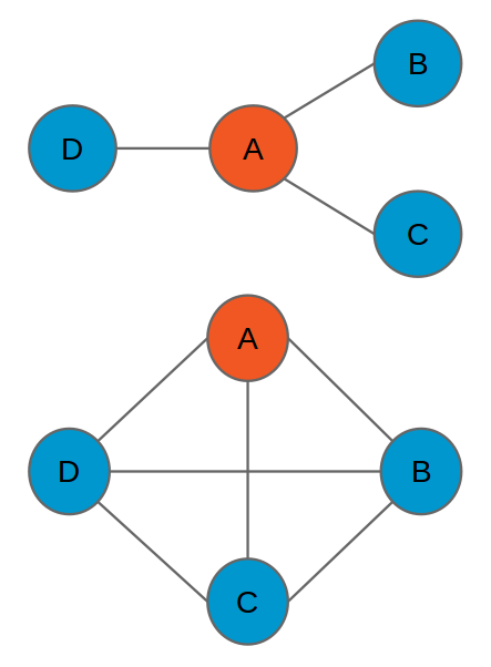
The number of triangles in a vertex's immediate neighborhood is a measure of the "density" of the vertex's neighborhood. In both of the figures below, vertex A has three immediate neighbors, ignoring edge directions. In the top figure, none of node A's neighbors is connected to any other neighbor, indicating a very loosely connected network. In contrast, all of the three neighbors are connected to each other in the bottom figure, indicating a tightly connected network.
tri = graphlab.triangle_counting.create(sg)
print tri.summary()
TriangleCountingModel
Graph:
+--------------+--------+
| num_edges    | 517127 |
| num_vertices | 233121 |
+--------------+--------+
Result:
+----------------+-------------------------------------------------------------------+
| graph          | SGraph. See m['graph']                                            |
| num_triangles  | 171968                                                            |
| triangle_count | SFrame with each vertex's triangle count. See m['triangle_count'] |
+----------------+-------------------------------------------------------------------+
Metric:
+---------------+-----------+
| training_time | 29.043092 |
+---------------+-----------+
Queriable Fields
+----------------+------------------------------------------------------------+
| Field          | Description                                                |
+----------------+------------------------------------------------------------+
| graph          | A new SGraph with the triangle count as a vertex property. |
| num_triangles  | Total number of triangles in the graph.                    |
| triangle_count | An SFrame with the triangle count for each vertex.         |
| training_time  | Total training time of the model                           |
+----------------+------------------------------------------------------------+
In this dataset, there is a lot of overlap between the companies with large influence in the Wikipedia article network (as measured by PageRank) and the companies with the largest and most dense neighborhoods, as measured by the triangle count method, but there are notable differences. ABC has only the sixth most triangles despite having the highest pagerank, while Microsoft ranks very high by both statistics, suggesting the Microsoft article is slightly more central in the network.
tri_out = tri['triangle_count']
print tri_out.topk('triangle_count', k=10)
+-------------------------------+----------------+
|              __id             | triangle_count |
+-------------------------------+----------------+
|           Microsoft           |     21447      |
|             Google            |     15491      |
|            Facebook           |     14200      |
|              IBM              |     11716      |
|       Paramount Pictures      |     10547      |
| American Broadcasting Company |     10514      |
|            Twitter            |      9219      |
|       Target Corporation      |      8474      |
|        Delta Air Lines        |      8195      |
|             Intel             |      7952      |
+-------------------------------+----------------+
[10 rows x 2 columns]
Single-source shortest path
Paths in a graph are a sequence of vertices, where each consecutive pair is connected by an edge in the graph. The single-source shortest path problem is to find the shortest path from all vertices in the graph to a user-specified target node. The source vertex with the smallest distribution of shortest paths can be considered the most central node in the graph.
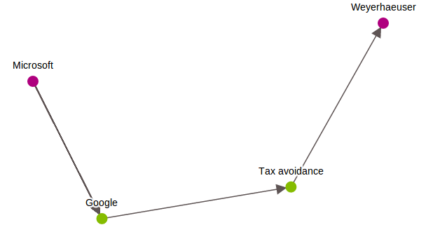
Because GraphLab Create SGraph's use directed edges, the shortest path toolkit also finds the shortest directed paths to a source vertex. In this example we find all shortest paths to the node for the Microsoft article, then visualize the shortest path from the Microsoft article to the Weyerhauser article. Interestingly, the quickest way to get from Microsoft to Weyerhauser is via the articles on Google and tax avoidance.
sssp = graphlab.shortest_path.create(sg, source_vid='Microsoft')
sssp.get_path(vid='Weyerhaeuser', show=True,
              highlight=['Microsoft', 'Weyerhaeuser'], arrows=True, ewidth=1.5)
[('Microsoft', 0.0),
 ('Google', 1.0),
 ('Tax avoidance', 2.0),
 ('Weyerhaeuser', 3.0)]