Time series
Data sources such as usage logs, sensor measurements, financial instruments, the presence of a time-stamp results in an implicit temporal ordering on the observations.
In these applications, it becomes important to be able to treat the time-stamp as an index around which several important operations such as:
- grouping the data with respect to various intervals of time
- aggregating data across time intervals
- aggregate/impute raw data into regular discrete intervals
The TimeSeries object is the fundamental data structure for multivariate time
series data. TimeSeries objects are backed by a single SFrame, but include
extra metadata.
| $$T$$ | $$V_1$$ | $$V_2$$ | $$...$$ | $$V_k$$ |
|---|---|---|---|---|
| $$t_{1}$$ | $$v_{11}$$ | $$v_{21}$$ | $$...$$ | $$v_{k1}$$ |
| $$t_{2}$$ | $$v_{12}$$ | $$v_{22}$$ | $$...$$ | $$v_{k2}$$ |
| $$t_{3}$$ | $$v_{13}$$ | $$v_{23}$$ | $$...$$ | $$v_{k3}$$ |
| $$...$$ | $$...$$ | $$...$$ | $$...$$ | $$...$$ |
| $$...$$ | $$...$$ | $$...$$ | $$...$$ | $$...$$ |
| $$t_{n}$$ | $$v_{1n}$$ | $$v_{2n}$$ | $$...$$ | $$v_{kn}$$ |
Each column pair $$(V_i, T)$$ in the table corresponds to a univariate time series. $$V_i$$ is the value column for $$T$$ is the index column that is shared among all the single (univariate) time series.
In this chapter, we will use a dataset obtained from the UCI machine learning repository. The dataset contains measurements of electric power consumption in one household with a one-minute sampling rate over a period of almost 4 years. The entire dataset contains around 2,075,259 measurements gathered between December 2006 and November 2010 (47 months). The dataset is stored as an SFrame that can be loaded as follows:
import graphlab as gl
household_data = gl.SFrame("http://s3.amazonaws.com/dato-datasets/household_electric_sample.sf")
Data:
+---------------------+-----------------------+---------+---------------------+
| Global_active_power | Global_reactive_power | Voltage |       DateTime      |
+---------------------+-----------------------+---------+---------------------+
|        4.216        |         0.418         |  234.84 | 2006-12-16 17:24:00 |
|        5.374        |         0.498         |  233.29 | 2006-12-16 17:26:00 |
|        3.666        |         0.528         |  235.68 | 2006-12-16 17:28:00 |
|         3.52        |         0.522         |  235.02 | 2006-12-16 17:29:00 |
|         3.7         |          0.52         |  235.22 | 2006-12-16 17:31:00 |
|        3.668        |          0.51         |  233.99 | 2006-12-16 17:32:00 |
|         3.27        |         0.152         |  236.73 | 2006-12-16 17:40:00 |
|        3.728        |          0.0          |  235.84 | 2006-12-16 17:43:00 |
|        5.894        |          0.0          |  232.69 | 2006-12-16 17:44:00 |
|        7.026        |          0.0          |  232.21 | 2006-12-16 17:46:00 |
+---------------------+-----------------------+---------+---------------------+
[1025260 rows x 4 columns]
Time series construction
We construct a TimeSeries object from the SFrame household_data by
specifying the DateTime column as the index column. The data is sorted by
the DateTime column when indexed into a time series.
household_ts = gl.TimeSeries(household_data, index="DateTime")
The index column of the TimeSeries is: DateTime
+---------------------+---------------------+-----------------------+---------+
|       DateTime      | Global_active_power | Global_reactive_power | Voltage |
+---------------------+---------------------+-----------------------+---------+
| 2006-12-16 17:24:00 |        4.216        |         0.418         |  234.84 |
| 2006-12-16 17:26:00 |        5.374        |         0.498         |  233.29 |
| 2006-12-16 17:28:00 |        3.666        |         0.528         |  235.68 |
| 2006-12-16 17:29:00 |         3.52        |         0.522         |  235.02 |
| 2006-12-16 17:31:00 |         3.7         |          0.52         |  235.22 |
| 2006-12-16 17:32:00 |        3.668        |          0.51         |  233.99 |
| 2006-12-16 17:40:00 |         3.27        |         0.152         |  236.73 |
| 2006-12-16 17:43:00 |        3.728        |          0.0          |  235.84 |
| 2006-12-16 17:44:00 |        5.894        |          0.0          |  232.69 |
| 2006-12-16 17:46:00 |        7.026        |          0.0          |  232.21 |
+---------------------+---------------------+-----------------------+---------+
[1025260 rows x 4 columns]
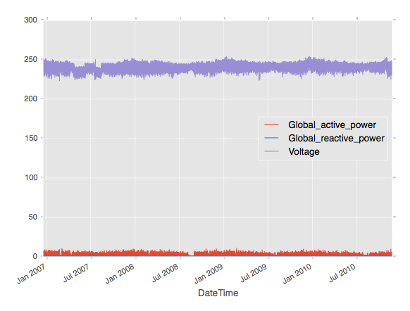
The following figure illustrates the multivariate time series. The index column
DateTime is the x-axis and the columns Global_active_power,
Global_reactive_power, and Voltage are illustrated in the y-axis.
Now, the dataset is indexed by the column Datetime and all future operations
involving time are now optimized. At any point of time, the time series can be
converted to an SFrame using the to_sframe function at zero cost.
sf = household_ts.to_sframe()
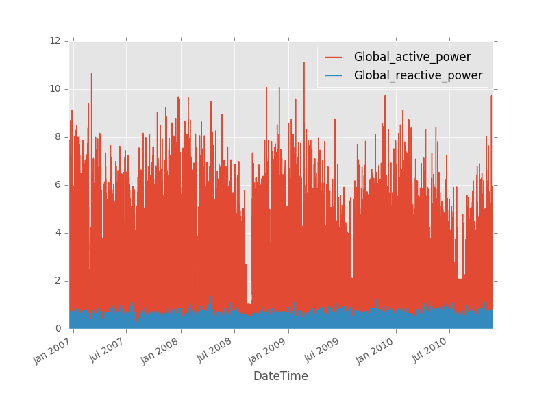
Note that each column in the TimeSeries object is an SArray. A subset
of columns can be selected as follows:
ts_power = household_ts[['Global_reactive_power', 'Global_reactive_power']]
The following figure illustrates the time series ts_power.
Resampling
In many practical time series analysis problems, we require observations to be over uniform time intervals. However, data is often in the form of non-uniform events with accompanying time stamps. As a result, one common prerequisite for time series applications is to convert an time series that is potentially irregularly sampled to one that is sampled at a regular frequency (or to a frequency different from the input data source).
There are three important primitive operations required for this purpose:
- Mapping – The operation which determines which time slice a specific observation belongs to.
- Interpolation/Upsampling – The operation used to fill in the missing values when there are no observations that map to a particular time slice.
- Aggregation/Downsampling –The operation used to aggregate multiple observations that below to the same time slice.
As an example, we resample the household_ts into a time-series at an hourly
granularity.
import datetime as dt

day = dt.timedelta(days = 1)
daily_ts = household_ts.resample(day, downsample_method='max', upsample_method=None)
+---------------------+---------------------+-----------------------+---------+
|       DateTime      | Global_active_power | Global_reactive_power | Voltage |
+---------------------+---------------------+-----------------------+---------+
| 2006-12-16 00:00:00 |        7.026        |         0.528         |  243.73 |
| 2006-12-17 00:00:00 |         6.58        |         0.582         |  249.07 |
| 2006-12-18 00:00:00 |        5.436        |         0.646         |  248.48 |
| 2006-12-19 00:00:00 |         7.84        |         0.606         |  248.89 |
| 2006-12-20 00:00:00 |        5.988        |         0.482         |  249.48 |
| 2006-12-21 00:00:00 |        5.614        |         0.688         |  247.08 |
| 2006-12-22 00:00:00 |        7.884        |         0.622         |  248.82 |
| 2006-12-23 00:00:00 |        8.698        |         0.724         |  246.77 |
| 2006-12-24 00:00:00 |        6.498        |         0.494         |  249.27 |
| 2006-12-25 00:00:00 |        6.702        |          0.7          |  250.62 |
+---------------------+---------------------+-----------------------+---------+
[1442 rows x 4 columns]
The following figure illustrates the resampled time series daily_ts.
In this example, the mapping is performed by choosing intervals of length
1 hour, the downsampling method is chosen by returning the maximum
value (for each column) of all the data points in the original time series, the
upsampling method sets a None value (for a column) corresponding to an
interval in the returned time series if there are no any values (for that
column) within that time interval in the original time series.
Shifting time series data
Time series data can also be shifted along the time dimension using the
TimeSeries.shift and TimeSeries.tshift methods.
The tshift operator shifts the index column of the time series along the time
dimension while keeping other columns intact. For example, we can shift the
household_ts by 5 mintues, so all the tuples by an hour:
interval = dt.timedelta(hours = 1)
shifted_ts = household_ts.tshift(interval)
+---------------------+---------------------+-----------------------+---------+
|       DateTime      | Global_active_power | Global_reactive_power | Voltage |
+---------------------+---------------------+-----------------------+---------+
| 2006-12-16 18:24:00 |        4.216        |         0.418         |  234.84 |
| 2006-12-16 18:26:00 |        5.374        |         0.498         |  233.29 |
| 2006-12-16 18:28:00 |        3.666        |         0.528         |  235.68 |
| 2006-12-16 18:29:00 |         3.52        |         0.522         |  235.02 |
| 2006-12-16 18:31:00 |         3.7         |          0.52         |  235.22 |
| 2006-12-16 18:32:00 |        3.668        |          0.51         |  233.99 |
| 2006-12-16 18:40:00 |         3.27        |         0.152         |  236.73 |
| 2006-12-16 18:43:00 |        3.728        |          0.0          |  235.84 |
| 2006-12-16 18:44:00 |        5.894        |          0.0          |  232.69 |
| 2006-12-16 18:46:00 |        7.026        |          0.0          |  232.21 |
+---------------------+---------------------+-----------------------+---------+
[1025260 rows x 8 columns]
The shift operator shifts forward/backward all the value columns while
keeping the index column intact. Notice that this operator does not change the
range of the TimeSeries object and it fills those edge tuples that lost their
value with None.
shifted_ts = household_ts.shift(steps = 3)
+---------------------+---------------------+-----------------------+---------+
|       DateTime      | Global_active_power | Global_reactive_power | Voltage |
+---------------------+---------------------+-----------------------+---------+
| 2006-12-16 17:24:00 |         None        |          None         |   None  |
| 2006-12-16 17:26:00 |         None        |          None         |   None  |
| 2006-12-16 17:28:00 |         None        |          None         |   None  |
| 2006-12-16 17:29:00 |        4.216        |         0.418         |  234.84 |
| 2006-12-16 17:31:00 |        5.374        |         0.498         |  233.29 |
| 2006-12-16 17:32:00 |        3.666        |         0.528         |  235.68 |
| 2006-12-16 17:40:00 |         3.52        |         0.522         |  235.02 |
| 2006-12-16 17:43:00 |         3.7         |          0.52         |  235.22 |
| 2006-12-16 17:44:00 |        3.668        |          0.51         |  233.99 |
| 2006-12-16 17:46:00 |         3.27        |         0.152         |  236.73 |
+---------------------+---------------------+-----------------------+---------+
[1025260 rows x 8 columns]
Index Join
Another important feature of TimeSeries objects in GraphLab Create is the
ability to efficiently join them across the index column. So far we created a
resampled TimeSeries from one of the electeric meters. Now is the time to join
the first resampled TimeSeries object ts1_resample_3m with the second
TimeSeries object electric_meter_ts2.
sf_other = gl.SFrame('http://s3.amazonaws.com/dato-datasets/household_electric_sample_2.sf')
ts_other = gl.TimeSeries(sf_other, index = 'DateTime')

household_ts.index_join(ts_other, how='inner')
+---------------------+---------------------+-----------------------+---------+
|       DateTime      | Global_active_power | Global_reactive_power | Voltage |
+---------------------+---------------------+-----------------------+---------+
| 2006-12-16 17:24:00 |        4.216        |         0.418         |  234.84 |
| 2006-12-16 17:26:00 |        5.374        |         0.498         |  233.29 |
| 2006-12-16 17:28:00 |        3.666        |         0.528         |  235.68 |
| 2006-12-16 17:29:00 |         3.52        |         0.522         |  235.02 |
| 2006-12-16 17:31:00 |         3.7         |          0.52         |  235.22 |
| 2006-12-16 17:32:00 |        3.668        |          0.51         |  233.99 |
| 2006-12-16 17:40:00 |         3.27        |         0.152         |  236.73 |
| 2006-12-16 17:43:00 |        3.728        |          0.0          |  235.84 |
| 2006-12-16 17:44:00 |        5.894        |          0.0          |  232.69 |
| 2006-12-16 17:46:00 |        7.026        |          0.0          |  232.21 |
+---------------------+---------------------+-----------------------+---------+
+------------------+
| Global_intensity |
+------------------+
|       18.4       |
|       23.0       |
|       15.8       |
|       15.0       |
|       15.8       |
|       15.8       |
|       13.8       |
|       16.4       |
|       25.4       |
|       30.6       |
+------------------+
[1025260 rows x 5 columns]
The how parameter in index_join operator determines the join method. The
acceptable values are 'inner','left','right', and 'outer'. The behavior is
exactly like the SFrame join methods.
Time series slicing
The range of a time series is defined as the interval (start, end) of the
time stamps that span the time series. It can be obtained as follows:
start_time, end_time = household_ts.range
(datetime.datetime(2006, 12, 16, 17, 24), datetime.datetime(2007, 11, 26, 20, 57))
We can obtain a slice of a time series that lies within its range using the
TimeSeries.slice operator.
import datetime as dt
start = dt.datetime(2006, 12, 16, 17, 24)
end = dt.datetime(2007, 11, 26, 21, 2)

sliced_ts = household_ts.slice(start, end)
+---------------------+---------------------+-----------------------+---------+
|       DateTime      | Global_active_power | Global_reactive_power | Voltage |
+---------------------+---------------------+-----------------------+---------+
| 2006-12-16 17:24:00 |        4.216        |         0.418         |  234.84 |
| 2006-12-16 17:26:00 |        5.374        |         0.498         |  233.29 |
| 2006-12-16 17:28:00 |        3.666        |         0.528         |  235.68 |
| 2006-12-16 17:29:00 |         3.52        |         0.522         |  235.02 |
| 2006-12-16 17:31:00 |         3.7         |          0.52         |  235.22 |
| 2006-12-16 17:32:00 |        3.668        |          0.51         |  233.99 |
| 2006-12-16 17:40:00 |         3.27        |         0.152         |  236.73 |
| 2006-12-16 17:43:00 |        3.728        |          0.0          |  235.84 |
| 2006-12-16 17:44:00 |        5.894        |          0.0          |  232.69 |
| 2006-12-16 17:46:00 |        7.026        |          0.0          |  232.21 |
+---------------------+---------------------+-----------------------+---------+
[246363 rows x 4 columns]
We can also slice the data for a particular year as follows:
start = dt.datetime(2010,1,1)
end  = dt.datetime(2011,1,1)
ts_2010 = household_ts.slice(start, end)
+---------------------+---------------------+-----------------------+---------+
|       DateTime      | Global_active_power | Global_reactive_power | Voltage |
+---------------------+---------------------+-----------------------+---------+
| 2010-01-01 00:00:00 |         1.79        |         0.236         |  240.65 |
| 2010-01-01 00:01:00 |         1.78        |         0.234         |  240.07 |
| 2010-01-01 00:03:00 |        1.746        |         0.186         |  240.26 |
| 2010-01-01 00:06:00 |         1.68        |          0.1          |  239.72 |
| 2010-01-01 00:07:00 |        1.688        |         0.102         |  240.34 |
| 2010-01-01 00:08:00 |        1.676        |         0.072         |  241.0  |
| 2010-01-01 00:11:00 |        1.618        |          0.0          |  240.11 |
| 2010-01-01 00:13:00 |        1.618        |          0.0          |  240.09 |
| 2010-01-01 00:14:00 |        1.622        |          0.0          |  240.38 |
| 2010-01-01 00:15:00 |        1.622        |          0.0          |  240.4  |
+---------------------+---------------------+-----------------------+---------+
[229027 rows x 4 columns]
Time series grouping
Quite often in time series analysis, we are required to split a single large time series in to groups of smaller time series grouped based on a property of the time stamp (e.g. per day of week).
The output of this operator is a graphlab.timeseries.GroupedTimeSeries
object, which can be used for retrieving one or more groups, or iterating
through all groups. Each group is a separate time series which possesses the
same columns as the original time series.
In this example, we group the time series household_ts by the day of the week.
household_ts_groups = household_ts.group(gl.TimeSeries.date_part.WEEKDAY)
print household_ts_groups.groups()
Rows: 7
[0, 1, 2, 3, 4, 5, 6]
household_ts_groups is a GroupedTimeSeries containing 7 groups where each
group is a single TimeSeries. In this example groups are named between 0 and 6
where 0 is Monday. We can access the data corresponding to a Monday as follows:
household_ts_monday = household_ts_groups.get_group(0)
+---------------------+---------------------+-----------------------+---------+
|       DateTime      | Global_active_power | Global_reactive_power | Voltage |
+---------------------+---------------------+-----------------------+---------+
| 2006-12-18 00:00:00 |        0.278        |         0.126         |  246.17 |
| 2006-12-18 00:03:00 |        0.206        |          0.0          |  245.94 |
| 2006-12-18 00:04:00 |        0.206        |          0.0          |  245.98 |
| 2006-12-18 00:06:00 |        0.204        |          0.0          |  245.22 |
| 2006-12-18 00:07:00 |        0.204        |          0.0          |  244.14 |
| 2006-12-18 00:08:00 |        0.212        |          0.0          |  244.0  |
| 2006-12-18 00:09:00 |        0.316        |         0.134         |  244.62 |
| 2006-12-18 00:10:00 |        0.308        |         0.132         |  244.61 |
| 2006-12-18 00:11:00 |        0.306        |         0.134         |  244.97 |
| 2006-12-18 00:12:00 |        0.306        |         0.136         |  245.51 |
+---------------------+---------------------+-----------------------+---------+
[146934 rows x 4 columns]
We can also iterate over all the groups in this GroupedTimeSeries object:
for name, group in household_ts_groups:
  print name, group
Time series union
We can also merge multiple time series into a single one using the union
operator. The merged time series is a valid time series with the time stamps
sorted correctly. In this example, we will use the union operator to re-unite
the time series that we split by the day of the week (using the group
operator).
household_ts_combined = household_ts_groups.get_group(0)
for i in range(1, 7):
  group = household_ts_groups.get_group(i)
  household_ts_combined = household_ts_combined.union(group)
+---------------------+---------------------+-----------------------+---------+
|       DateTime      | Global_active_power | Global_reactive_power | Voltage |
+---------------------+---------------------+-----------------------+---------+
| 2006-12-16 17:24:00 |        4.216        |         0.418         |  234.84 |
| 2006-12-16 17:26:00 |        5.374        |         0.498         |  233.29 |
| 2006-12-16 17:28:00 |        3.666        |         0.528         |  235.68 |
| 2006-12-16 17:29:00 |         3.52        |         0.522         |  235.02 |
| 2006-12-16 17:31:00 |         3.7         |          0.52         |  235.22 |
| 2006-12-16 17:32:00 |        3.668        |          0.51         |  233.99 |
| 2006-12-16 17:40:00 |         3.27        |         0.152         |  236.73 |
| 2006-12-16 17:43:00 |        3.728        |          0.0          |  235.84 |
| 2006-12-16 17:44:00 |        5.894        |          0.0          |  232.69 |
| 2006-12-16 17:46:00 |        7.026        |          0.0          |  232.21 |
+---------------------+---------------------+-----------------------+---------+
[1025260 rows x 4 columns]
Common operations with SFrame/SArray
Because the time series data structure is backed by an SFrame, there are many operations that behave exactly like the SFrame. These include
- Logical filters (row selection)
- SArray apply functions (univariate user defined functions UDFs)
- Time series apply functions (multivariate UDFs)
- Selecting columns
- Adding, removing, and swapping columns
- Head, tail, row range selection
- Joins (on the non-index column)
See the chapter on SFrame for more usage details on the above functions.
Save and Load
Just like every other object, the time series can be saved and loaded as follows:
household_ts.save("/tmp/first_copy")
household_ts_copy = graphlab.TimeSeries("/tmp/first_copy")